Linear Models

Most basic statistical model.
Analyzes the relationship between a response variable and a set of explanatory variables.
Predict unknown values

Assumptions of Regression Line

Linearity - The relationship between X and Y is linear
Independence of Errors - Error values are statistically independent
Normality of Error - Error values are normally distributed for any given value of X
Equal variance - The probability distribution of the error has constant variance

Residuals are the difference between predicted and actual values

Steps in generating a regression model

Gather sample of observed values
Create a linear model using lm()
Find the coefficient from the model using coefficients(lm)
Extract summary of relationship summary(lm) and residuals(lm)
Use predict(lm, df) to predict the values for a new set of predictor variables

Simple Linear Regression

$y = ax + b$

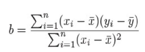
$a=ybar - b*xbar$

lm(formula, data, subset, weights, na.action, method="qr", model=TRUE, x = FALSE, y = FALSE, qr = TRUE, singular.ok = TRUE, contrasts = NULL, offset, ...) 

#model determines whether to return model frame
#x and y determines whether to return model matrix of response vector should be returned or not
#generates a model using ordinary least squares for the given formula

Symbol	Usage
~	Separates response variable from explanatory variable
+	Separates predictor variables
:	Represents interaction between predictor variables
*	Shortcut to represent all possible interactions
^ n	Represents Interaction upto degree n
.	Placeholder representing all other variables
-	Used to remove a predictor variable from the equation
-1	Forces the line through the origin x = 0
I() Identity Function	Element within the parenthesis are interpreted arithmetically
function	Mathematical function are also be used directly in formulae

Polynomial Regression

The relationship is modelled as an $nth$ order polynomial
```
poly(x, ..., degree=n, coefs=NULL, raw=FALSE)
```

Multiple Linear

The response variable is predicted from two or more explanatory variables

Multilevel

Predicting the response variable from data that have a hierarchical structure

Multivariate

Predicting the value of multiple response variables

Cox Proportional Hazards & Time Series

Prediction of time

Resistant Regression

Done by using least median squares (LMS) or least trimmed squares (LTS) estimators

lqs(formula, data, method=c("LMS", "LTS"))

Robust Regression

rlm(formula, data, weights, subset, na.action, method=c("M", "MM", "model.frame"), wt.method=c("inv.var", "case"), model=TRUE, x.ret = TRUE, y.ret = FALSE, contrasts = NULL)

Regression Analysis Types

Type	Definition
Nonlinear	Prediction of the response variable whose values in non linear
Nonparametric	The form of the model is derived from the data and not mentioned a priori
Robust	The values of response variable in this approach is resistant to the effect of influential observations

Summarizing and extracting data from linear model

Function	Action
summary()	Displays details results for the fitted model
coefficients()	Lists out the model parameters for the fitted model
confint()	Provides confidence intervals for the model parameters
fitted()	Lists the predicted values in a fitted model
residuals	Lists the residual values in a fitted model
anova(lm,…,scale=0,test=”F”)	Generates an ANOVA table for the fitted model
vcov(lm,…)	Lists the covariance matrix for model parameters
AIC()	Prints Akaike’s Information Criterion
plot()	Generates plots for evaluation model fitness
predict()	Uses the fitted model to predict the response variables for a new dataset
influence()	Describes the influence of various features
influence.measures()	Describes the influence in a easier to interpret way

Analyzing the fit of the model

Residuals-difference between predicted values and the observed
```
R^2= explained variation of model / total variation of model
```
for models that fit the data well the R^2 will be near 0
1. residuals(object, ...): Computes the vector of residuals from a fitted model object.

fitted(object, ...): Calculates the vector of fitted values from a fitted model object.
predict(object, newdata, ...): Generates predictions using a fitted model object and new data.
confint(object, parm, ...): Computes confidence intervals for the coefficients in the fitted model object.
influence(model, ...): Calculates the influence of different parameters in the fitted model object.
vcov(object, ...): Computes the variance-covariance matrix from the linear model object.

Visualizing the data

model<- lm(y ~ x)
plot(y,x,abline(lm(x~y)))

plot(model) shows

Residuals vs. fitted values: Shows the relationship between residuals and predicted values to identify patterns or deviations.
Normal Q-Q plot: Compares the residuals to the expected values under a normal distribution assumption.
Scale-location plot: Displays the square root of the absolute residuals against fitted values to assess variance homogeneity.
Residuals vs. leverages plot: Examines the relationship between standardized residuals and leverage values.

Refitting a model

lmnew <- update(lm, formula)

detect influential points

outliers - detected based on finding the cook.distance between each of them

Assumptions of Least Squares Regression

Linearity - Relation between response and predictor is linear
Full Rank - No relationship exists between predictor variables
1. If correlation exists between predictor use principal components regression
Exogeneity of predictor variables - The expected value of $epsilon=0$ for all predictor variables
1. Test using ncvTest()
Homoscedasticity - The variable of $epsilon$ is constant and not correlation with predictor variables
1. Use robust or resistant regression function if model is homoscedastic
Non autocorrelation - The values of y are not correlated in a sequence of observations
1. Test using durbin.watson
Exogenously generated data - The predictor variables are generated independently of the process that generated $epsilon$
The error term $epsilon$ is normally distributed with standard deviation $sigma$ and $mean=0$
1. If error isn’t normal use ridge regression

Generalized Linear Models

Logistic Regression

Prediction of a categorical response from the given explanatory variables
Predict a binary outcome from a set of numeric variables
```
glm(formula, data, family=binomial(link="logit"))
```

Poisson Regression

Prediction of the response variable from the counts for one or more explanatory variables

Nonlinear Least Squares

nlm(formula, data, start, control=nls.control(), algorithm=c("default", "plinear", "port"),trace=FALSE,subset,weights,na.action,model=FALSE,lower=-Inf,upper=Inf,...)

#start contains starting estimates for the fit
#control contains list of arguments for controlling the fitting process
#algorithm plinear-golub_pereya, port-nl2sol
#trace whether to print process of training
#lower and upper sets lower and upper bounds for the model resp...

Questions

Question 1: Describe the lm() function in R with all of its parameters.

In R, the lm() function is used to fit linear regression models. It stands for “linear model.” This function takes several parameters to specify the model formula, data, and additional options. Here is a description of the parameters:

formula: This parameter specifies the relationship between the dependent variable and the independent variables in the form of a formula. It typically follows the syntax y ~ x1 + x2 + ..., where y is the dependent variable, and x1, x2, etc., are the independent variables.
data: This parameter specifies the data frame or list that contains the variables in the formula. It is used to look up the variables used in the formula.
subset (optional): This parameter allows you to specify a subset of the data to be used in the model fitting. It takes a logical expression that determines which observations to include.
weights (optional): This parameter is used to specify a vector of weights for the observations. It allows you to assign different weights to individual data points, influencing their importance in the model fitting.
na.action (optional): This parameter specifies what should be done with missing values in the data. It can take values such as na.omit to omit any observations with missing values or na.exclude to include them with missing values.
method (optional): This parameter allows you to specify the method to be used for fitting the linear model. By default, it is set to "qr", which uses the QR decomposition method. Other options include "model.frame" and "model.matrix", which return the model frame and model matrix, respectively, without fitting the model.
model (optional): This parameter is used to specify a previously fitted model to extract the model frame and use it for fitting a new model.
x (optional): This parameter allows you to provide a model matrix or data frame containing the independent variables directly, instead of using the formula and data parameters.
y (optional): This parameter allows you to provide the dependent variable directly, instead of using the formula and data parameters.
qr (optional): This parameter is used to specify a QR decomposition object. It allows you to provide a precomputed QR decomposition for faster model fitting.
singular.ok (optional): This parameter specifies whether the model fitting should continue even if the model matrix is singular. By default, it is set to FALSE, and an error is raised if singularity is detected.
contrasts (optional): This parameter allows you to specify how categorical variables should be contrasted. It can be set to a list that defines the contrast functions for different variables.

These are the main parameters of the lm() function in R. Depending on your specific needs, you can adjust these parameters to customize the linear regression model fitting process.

Question 2: What is a model matrix?

A model matrix, also known as a design matrix, is a matrix that represents the design or structure of a statistical model. It is used in various statistical modeling techniques, including linear regression.

In the context of linear regression, a model matrix is constructed by transforming the predictor variables (independent variables) into a matrix format that can be used for modeling. Each column of the model matrix represents a predictor variable, and each row represents an observation or data point.

The purpose of creating a model matrix is to encode the predictor variables in a way that can be easily used in the regression model. This encoding typically involves converting categorical variables into a set of binary indicator variables, also known as dummy variables.

For example, let’s say we have a linear regression model with a single predictor variable, x, and an intercept term. If x is a continuous variable, the model matrix would consist of two columns: one for the intercept (which is a constant value of 1 for all observations) and one for x, with each row containing the corresponding values of the intercept and x for each observation.

If x is a categorical variable with three levels (e.g., “A”, “B”, “C”), the model matrix would consist of four columns: one for the intercept and three dummy variables representing the levels of x. Each dummy variable would take the value of 1 if the corresponding level is present for that observation and 0 otherwise.

The model matrix is used by the regression algorithm to estimate the coefficients for each predictor variable and the intercept term. It provides a structured representation of the predictor variables that can be easily manipulated and used for model fitting and inference.

In R, the model.matrix() function can be used to generate the model matrix based on a formula and a data frame. It automatically handles the encoding of categorical variables into dummy variables and creates the appropriate design matrix for the specified model.

Question 3: Describe the rlm() function and its parameters.

In R, the rlm() function is used to fit robust linear regression models. It stands for “robust linear model.” This function is specifically designed to handle data that may contain outliers or violations of the assumptions of ordinary least squares regression. The rlm() function is part of the MASS package, so you need to load the package before using it. Here is a description of its parameters:

formula: This parameter specifies the relationship between the dependent variable and the independent variables in the form of a formula. It follows the same syntax as in the lm() function, using the tilde (~) operator.
data: This parameter specifies the data frame or list that contains the variables in the formula. It is used to look up the variables used in the formula.
subset (optional): This parameter allows you to specify a subset of the data to be used in the model fitting. It takes a logical expression that determines which observations to include.
weights (optional): This parameter is used to specify a vector of weights for the observations. It allows you to assign different weights to individual data points, influencing their importance in the model fitting.
control (optional): This parameter is used to control the behavior of the rlm() function through a list of control parameters. These parameters include options such as the convergence criteria, tuning constants, and the maximum number of iterations.
method (optional): This parameter allows you to specify the method to be used for fitting the robust linear model. By default, it is set to "M" for M-estimation. Other options include "MM" for MM-estimation and "LTS" for Least Trimmed Squares estimation.
model (optional): This parameter is used to specify a previously fitted model to extract the model frame and use it for fitting a new model.
x (optional): This parameter allows you to provide a model matrix or data frame containing the independent variables directly, instead of using the formula and data parameters.
y (optional): This parameter allows you to provide the dependent variable directly, instead of using the formula and data parameters.

The rlm() function in R fits robust linear regression models by minimizing robust scale estimates, such as M-estimators or MM-estimators, to provide more robustness against outliers or violations of assumptions. It is particularly useful when dealing with data that may have influential observations or non-normal error distributions.

Question 4: Describe the nlm() function and its parameters.

In R, the nlm() function is used for minimizing a function of several variables using a Newton-type algorithm. It stands for “Newton-like minimization.” This function is primarily used for unconstrained optimization problems where you need to find the minimum of a given objective function. Here is a description of its parameters:

p: This parameter specifies the starting values for the optimization process. It represents a numeric vector or matrix of initial values for the variables being optimized.
fn: This parameter specifies the objective function to be minimized. It should be a function that takes the vector of variables as its argument and returns a scalar value representing the objective function evaluated at that point.
...: This parameter allows for additional arguments to be passed to the objective function (fn).
hessian (optional): This parameter determines whether the Hessian matrix should be computed and returned. By default, it is set to FALSE. Setting it to TRUE returns the Hessian matrix, which is the matrix of second partial derivatives of the objective function.
...: This parameter allows for additional arguments to be passed to the optimization function.

The nlm() function uses a variant of Newton’s method, called the Newton–Raphson method, to iteratively approximate the minimum of the objective function. It starts from the initial values provided in p and updates the values at each iteration using the first and second derivatives of the objective function.

The function fn should be a user-defined function that takes the vector of variables as input and returns a scalar value. The goal is to find the values of the variables that minimize this function. You can also pass additional arguments to fn using the ... parameter.

The nlm() function returns a list containing information about the optimization process, including the estimated minimum, the vector of variables at the minimum, and the convergence status. If the hessian parameter is set to TRUE, the Hessian matrix will also be included in the output.

It’s worth noting that the nlm() function is typically used for local optimization problems and may not guarantee finding the global minimum. If you are dealing with global optimization, you might need to consider other optimization algorithms or packages in R, such as optim(), which allows for more flexible optimization routines.